段首语
此系列文章用来做R语言的学习,以及对于使用R语言进行数据处理和作图的代码汇总,方便大家随时进行查找、使用。
一、base R 基础作图
图形创建
- 颜色准备
1
library(RColorBrewer)
- 直方图 histogram
1
2
data(VADeaths)
hist(VADeaths,breaks=10, col=brewer.pal(3,"Set3"),main="Set3 3 colors")

- 线性图 line chart
1
plot(AirPassengers,type="l")

- 柱状图 bar chart
1
barplot(iris$Petal.Length) #Creating simple Bar Graph

1
barplot(table(iris$Species,iris$Sepal.Length),col = brewer.pal(3,"Set1"))

- 盒形图 boxplot
1
2
data(iris)
boxplot(iris$Sepal.Length,col="red")

1
boxplot(iris$Sepal.Length~iris$Species,col=topo.colors(3,alpha = 0.8))

- 散点图
1
plot(x=iris$Petal.Length)

1
plot(x=iris$Petal.Length,y=iris$Species)

1
plot(iris,col=brewer.pal(3,"Set1"))

- 六边形密度图 Hexbin Binning
1
2
3
4
5
library(hexbin)
library(ggplot2)
diamonds <- diamonds
a=hexbin(diamonds$price,diamonds$carat,xbins=40)
plot(a)

1
2
3
4
rf <- colorRampPalette(rev(brewer.pal(40,'Set3')))
## Warning in brewer.pal(40, "Set3"): n too large, allowed maximum for palette Set3 is 12
## Returning the palette you asked for with that many colors
hexbinplot(diamonds$price~diamonds$carat, data=diamonds, colramp=rf)

*马赛克图(Mosaic Plot),也叫做不等宽柱状图(Marimekko Chart)
1
2
data(HairEyeColor)
mosaicplot(HairEyeColor)

- 热图
1
2
3
4
5
6
7
8
9
head(mtcars)
##                    mpg cyl disp  hp drat    wt  qsec vs am gear carb
## Mazda RX4         21.0   6  160 110 3.90 2.620 16.46  0  1    4    4
## Mazda RX4 Wag     21.0   6  160 110 3.90 2.875 17.02  0  1    4    4
## Datsun 710        22.8   4  108  93 3.85 2.320 18.61  1  1    4    1
## Hornet 4 Drive    21.4   6  258 110 3.08 3.215 19.44  1  0    3    1
## Hornet Sportabout 18.7   8  360 175 3.15 3.440 17.02  0  0    3    2
## Valiant           18.1   6  225 105 2.76 3.460 20.22  1  0    3    1
heatmap(as.matrix(mtcars))

- 地图 Map
1
2
3
4
5
6
7
8
## devtools::install_github("rstudio/leaflet")
library(magrittr)
library(leaflet)
m <- leaflet() %>%
  addTiles() %>% # Add default OpenStreetMap map tiles
  addMarkers(lng=77.2310, lat=28.6560, popup="food of chandni chowk")
m
## Error in loadNamespace(name): there is no package called 'webshot'
- 3D
1
2
3
4
5
6
7
8
9
10
11
12
13
data(iris, package="datasets")
library(car)
# scatter3d(Petal.Width~Petal.Length+Sepal.Length|Species, data=iris, fit="linear",residuals=TRUE, parallel=FALSE, bg="black", axis.scales=TRUE, grid=TRUE, ellipsoid=FALSE)

library(lattice)
attach(iris)# 3d scatterplot by factor level
## The following objects are masked from iris (pos = 4):
##
##     Petal.Length, Petal.Width, Sepal.Length, Sepal.Width, Species
## The following objects are masked from iris (pos = 6):
##
##     Petal.Length, Petal.Width, Sepal.Length, Sepal.Width, Species
  cloud(Sepal.Length~Sepal.Width*Petal.Length|Species, main="3D Scatterplot by Species")

1
  xyplot(Sepal.Width ~ Sepal.Length, iris, groups = iris$Species, pch= 20)

- 相关性图 Correlogram (GUIs)
1
2
3
4
5
6
7
8
cor(iris[1:4])
##              Sepal.Length Sepal.Width Petal.Length Petal.Width
## Sepal.Length    1.0000000  -0.1175698    0.8717538   0.8179411
## Sepal.Width    -0.1175698   1.0000000   -0.4284401  -0.3661259
## Petal.Length    0.8717538  -0.4284401    1.0000000   0.9628654
## Petal.Width     0.8179411  -0.3661259    0.9628654   1.0000000
library(corrgram)
corrgram(iris)

图形定制
1.字符、文本
- 文字大小
| 参数 | 描述 |
|---|---|
| cex | 相对于默认大小的缩放倍数 |
| cex.axis | 坐标轴刻度文字的缩放倍数 |
| cex.lab | 坐标轴标签的缩放倍数 |
| cex.main | 标题的缩放倍数 |
| cex.sub | 副标题的缩放倍数 |
- 文字字体
| 参数 | 描述 |
|---|---|
| font | 用于指定绘图所用的字体样式。1=常规,2=粗体,3=斜体,4=粗斜体,5=符号字体(以Adobe符号编码表示) |
| font.axis | 坐标轴刻度字体样式 |
| font.lab | 坐标轴标签字体样式 |
| font.main | 标题的字体样式 |
| font.sub | 副标题的字体样式 |
| ps | 字体磅值,文本的最终大小为ps*cex |
| family | 绘制文本时使用的字体族,serif(衬线),sans(无衬线),mono(等宽) |
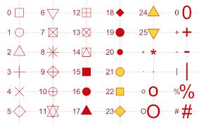
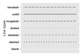
2.符号和线条
| 参数 | 描述 |
|---|---|
| pch | 符号类型 |
| cex | 符号大小 |
| lty | 线条类型 |
| lwd | 线条宽度 |
1
2
3
dose <- c(20,30,40,50,60)
drugA <- c(16,20,28,40,60)
plot(dose,drugA,type = "b",lty=3,lwd=3,pch=15,cex=2)

3.颜色
| 参数 | 描述 |
|---|---|
| col | 默认绘图颜色 |
| col.axis | 坐标轴刻度文字颜色 |
| col.lab | 坐标轴标签文字颜色 |
| col.main | 标题颜色 |
| col.sub | 副标题颜色 |
| fg | 图形的前景色 |
| bg | 图形的后景色 |
- 使用颜色下标、名称,十六进制、RGB、或者HSV表示
col=1,col=”white”,col=#FFFFFF”.col=rgb(1,1,1)和col=hsv(0,0,1)
- 函数
1
2
3
4
5
6
7
8
9
10
11
12
13
14
15
16
17
18
19
20
21
22
23
24
## colors() 可返回所有可用的颜色名称
head(colors())
## [1] "white"         "aliceblue"     "antiquewhite"  "antiquewhite1"
## [5] "antiquewhite2" "antiquewhite3"

rainbow(10)
##  [1] "#FF0000" "#FF9900" "#CCFF00" "#33FF00" "#00FF66" "#00FFFF" "#0066FF"
##  [8] "#3300FF" "#CC00FF" "#FF0099"

heat.colors(10)
##  [1] "#FF0000" "#FF2400" "#FF4900" "#FF6D00" "#FF9200" "#FFB600" "#FFDB00"
##  [8] "#FFFF00" "#FFFF40" "#FFFFBF"

terrain.colors(10)
##  [1] "#00A600" "#2DB600" "#63C600" "#A0D600" "#E6E600" "#E8C32E" "#EBB25E"
##  [8] "#EDB48E" "#F0C9C0" "#F2F2F2"

topo.colors(10)
##  [1] "#4C00FF" "#0019FF" "#0080FF" "#00E5FF" "#00FF4D" "#4DFF00" "#E6FF00"
##  [8] "#FFFF00" "#FFDE59" "#FFE0B3"

cm.colors(10)
##  [1] "#80FFFF" "#99FFFF" "#B3FFFF" "#CCFFFF" "#E6FFFF" "#FFE6FF" "#FFCCFF"
##  [8] "#FFB3FF" "#FF99FF" "#FF80FF"
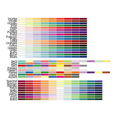
- R 包
RColorBrewer
1
2
3
4
5
6
7
8
9
10
11
12
13
14
15
16
17
18
19
20
21
22
23
24
25
26
27
28
29
30
31
32
33
34
35
36
37
38
39
library(RColorBrewer)
brewer.pal.info ## 展示所有颜色
##          maxcolors category colorblind
## BrBG            11      div       TRUE
## PiYG            11      div       TRUE
## PRGn            11      div       TRUE
## PuOr            11      div       TRUE
## RdBu            11      div       TRUE
## RdGy            11      div      FALSE
## RdYlBu          11      div       TRUE
## RdYlGn          11      div      FALSE
## Spectral        11      div      FALSE
## Accent           8     qual      FALSE
## Dark2            8     qual       TRUE
## Paired          12     qual       TRUE
## Pastel1          9     qual      FALSE
## Pastel2          8     qual      FALSE
## Set1             9     qual      FALSE
## Set2             8     qual       TRUE
## Set3            12     qual      FALSE
## Blues            9      seq       TRUE
## BuGn             9      seq       TRUE
## BuPu             9      seq       TRUE
## GnBu             9      seq       TRUE
## Greens           9      seq       TRUE
## Greys            9      seq       TRUE
## Oranges          9      seq       TRUE
## OrRd             9      seq       TRUE
## PuBu             9      seq       TRUE
## PuBuGn           9      seq       TRUE
## PuRd             9      seq       TRUE
## Purples          9      seq       TRUE
## RdPu             9      seq       TRUE
## Reds             9      seq       TRUE
## YlGn             9      seq       TRUE
## YlGnBu           9      seq       TRUE
## YlOrBr           9      seq       TRUE
## YlOrRd           9      seq       TRUE
display.brewer.all() ## 打开调色板
1
2
3
mycolor <- brewer.pal(5,"Set1") ## 调用颜色
mycolor
## [1] "#E41A1C" "#377EB8" "#4DAF4A" "#984EA3" "#FF7F00"
4.图形尺寸和边界尺寸
| 参数 | 描述 |
|---|---|
| pin | 以英寸表示图形尺寸 |
| mai | 以数值向量表示边界大小,“下,左,上,右”,单位英寸 |
| mar | 以数值向量表示边界大小,“下,左,上,右”,单位英分 |
5.标题
title()
1
title(main="main title",sub= "sub title",xlab = "x-axis lable",ylab = "y-axis lable")
6.坐标轴
axis()
1
axis(side,at = ,labels = ,pos = ,lty = ,col = ,Las=,tck=, ……)
| side | 整数,表示绘制坐标轴的位置(1=下,2=左,3=上,4=右) |
| at | 数值型向量,表示需要绘制刻度线的位置 |
| labels | 字符型向量,表示置于刻度线旁边的文字标签,(如果为Null,则默认使用at()中的值 |
| pos | 坐标轴线绘制位置的坐标(相交点的坐标)| |
| lty | 线条类型 |
| col | 线条颜色与刻度线颜色 |
| las | 标签是否平行于(=0)或垂直于(=2)坐标轴(标签值较长的情况) |
| tck | 刻度线长度,负数为外侧,正数为内侧,0表示禁用,1表示绘制网格线,默认-0.01 |
| xlim | x轴的范围 |
| ylim | y轴的范围 |
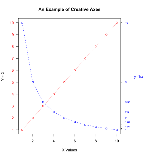
axes=FALSE 禁用坐标轴, yaxt=”n”,xaxt=”n” 分别禁用y轴和x轴
1
2
3
4
5
6
7
8
9
10
11
12
13
14
## 举例

x <- c(1:10)
y <- x
z <- 10/x
opar <- par(no.readonly = T)

par(mar=c(5,4,4,8)+0.1)
plot(x,y,type="b",pch=21,col="red",yaxt="n",lty=3,ann=FALSE)
lines(x,z,type="b",pch=22,col="blue",lty=2)
axis(2,at=x,labels = x,col.axis="red",las=2)
axis(4,at=z,labels = round(z,digits = 2),col.axis="blue",las=2,cex.axis=0.7,tck=-0.01)
mtext("y=1/x",side=4,line=3,cex.lab=1,las=2,col="blue")
title("An Example of Creative Axes",xlab = "X Values",ylab = "Y = X")
1
par(opar)
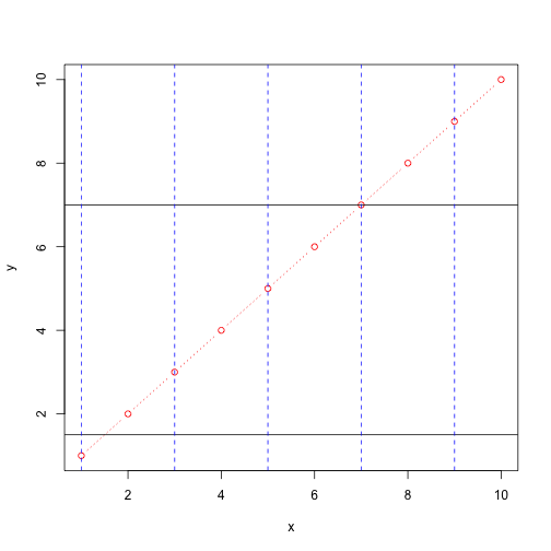
7.参考线
abline(h=yvalues,v=xvalues)为图形添加参考线
1
2
3
plot(x,y,type="b",pch=21,col="red",lty=3)
abline(h=c(1.5,7))
abline(v=seq(1,10,2),lty=2,col="blue")
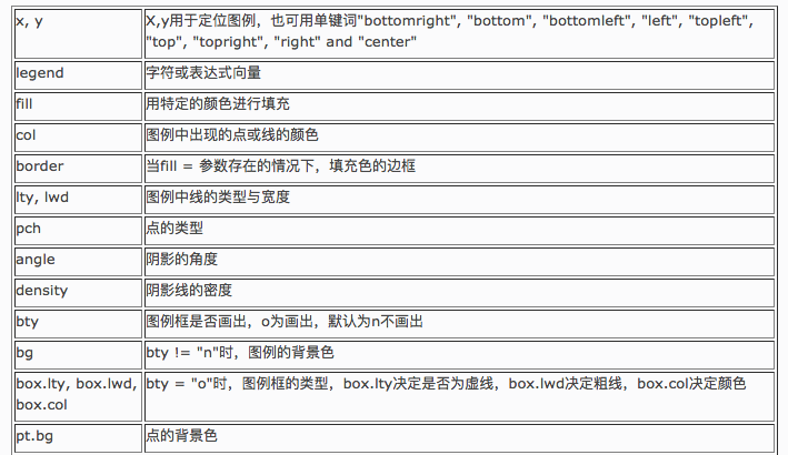
8.图例
legend(location,title,legend,…)
| 选项 | 描述 |
|---|---|
| location | 1,指定坐标;2,使用关键字(bottom,topright 等),可同时使用inset=指定向图形内侧移动的大小 |
| title | 标题 |
| legend | 标签 |

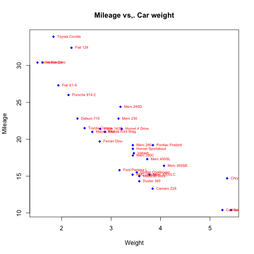
9.文本标注
text(location,”text to place”,pos,…) mtext(“text to place”,side,line=n,…)
| 选项 | 描述 |
|---|---|
| location | 文本位置 |
| pos | 相对于位置的方位,1=下,2=左,3=上,4=右,使用offset=指定偏移量 |
| side | 文本的边,lines=内移或外移文本,adj=0文本左下对齐,adj=1右上对齐 |
1
attach(mtcars)
1
2
3
## The following object is masked from package:ggplot2:
##
##     mpg
1
2
3
4
5
6
7
plot(wt,mpg,
     main = "Mileage vs,. Car weight",
     xlab = "Weight",ylab = "Mileage",
     pch=18,col="blue")
text(wt,mpg,
     row.names(mtcars),
     cex=0.6,pos=4,col = "red")
1
detach(mtcars)
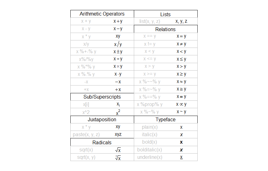
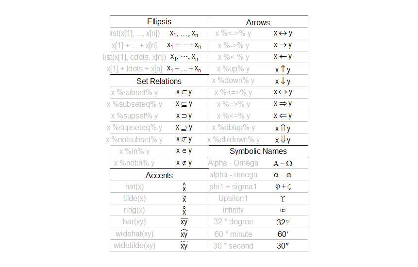
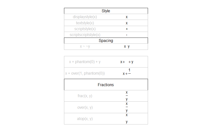
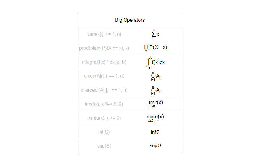
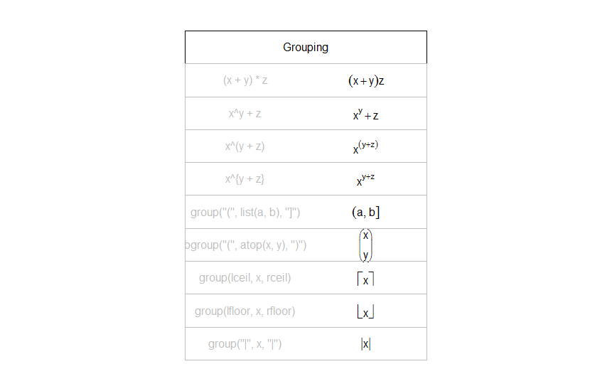
10.数学标注
plotmath()添加数学符号
11.图形的组合
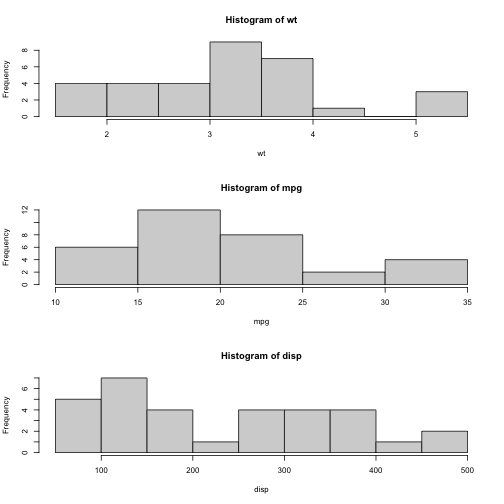
- par()
使用参数mfrow=c(nrows,ncols) or mfcol=c(nrows,ncols)
1
attach(mtcars)
1
2
3
## The following object is masked from package:ggplot2:
##
##     mpg
1
2
3
4
5
opar <- par(no.readonly = T)
par(mfrow=c(3,1))
hist(wt)
hist(mpg)
hist(disp)
1
2
par(opar)
detach(mtcars)
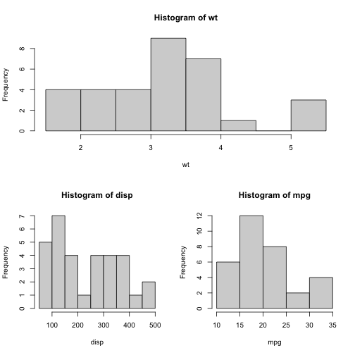
- layout()
layout(mat),使用mat指定图形位置(所在行)
1
attach(mtcars)
1
2
3
## The following object is masked from package:ggplot2:
##
##     mpg
1
2
3
4
layout(matrix(c(1,1,2,3),2,2,byrow = T))
hist(wt)
hist(disp)
hist(mpg)
1
detach(mtcars)
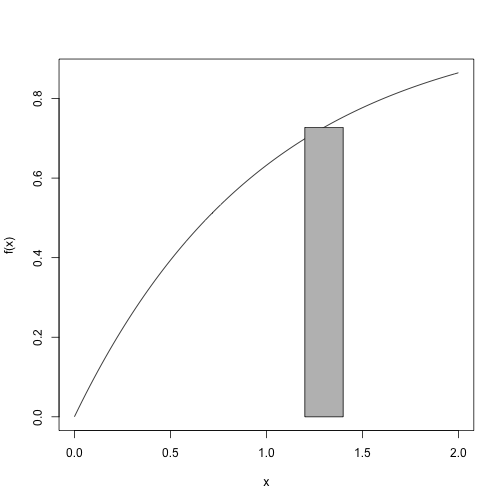
12.添加多边形
polygon()
1
2
3
f <- function(x) return(1-exp(-x))
curve(f,0,2)
polygon(c(1.2,1.4,1.4,1.2),c(0,0,f(1.3),f(1.3)),col = "gray")
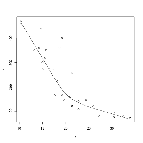
13.平滑散点
lowess() 与 loess() 函数
1
2
3
datatest <- data.frame(x=mtcars$mpg,y=mtcars$disp)
plot(datatest)+
lines(lowess(datatest))
1
## integer(0)
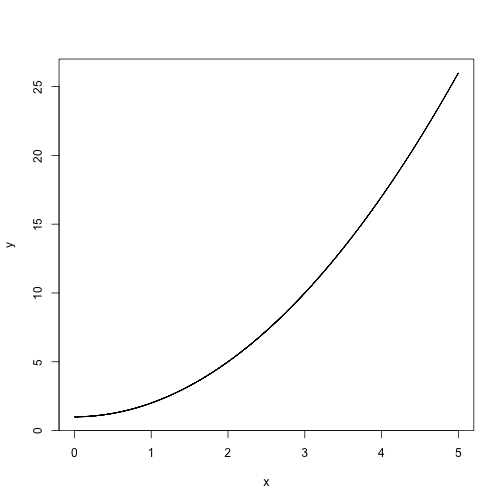
14.绘制显式表达式的函数
对于具有一定函数关系的曲线图的绘制
1、将其中的数抽样进行plot
1
2
3
4
g <- function(t) {return (t^2+1)^0.5 }
x <- seq(0,5,length=10000)
y <- g(x)
plot(x,y,type="l")
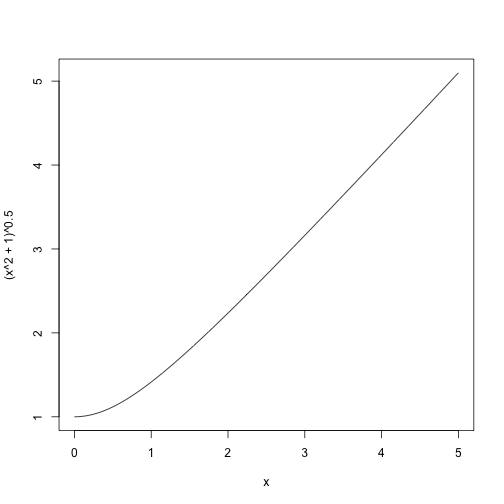
2、直接绘制函数图像(add=T,在原有图形上添加)
1
curve((x^2+1)^0.5,0,5)
二、ggplot2作图
ggplot2的基本语法
ggplot2(data = ) +
< GEOM_FUNCTION >( mapping = aes(< MAPPINGS >),stat=< STAT >,position = < POSITION >)+
1
2
3
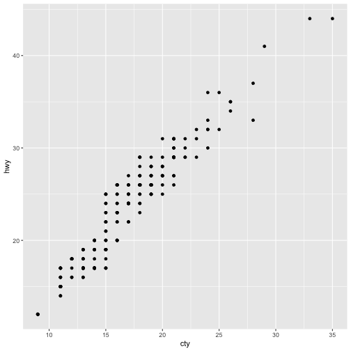
library(ggplot2)
## 写法一
ggplot(data = mpg,aes(x = cty,y = hwy)) + geom_point()

1
2
## 写法二
qplot(x = cty,y = hwy,data = mpg,geom = "point")

1
2
3
## 保存
ggsave("plot.png",width = 5,height = 5)
last_plot() ## 显示最后一张图
基本图类型
1.基础图块
1
2
3
4
5
6
7
8
9
10
11
12
13
14
15
16
17
18
19
20
21
22
23
24
25
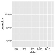
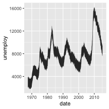
a <- ggplot(economics,aes(date,unemploy))
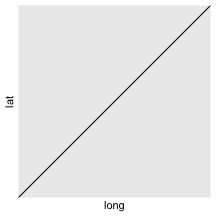
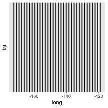
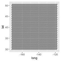
b <- ggplot(seals,aes(x=long,y=lat))
head(economics)
## # A tibble: 6 × 6
## date pce pop psavert uempmed unemploy
## <date> <dbl> <dbl> <dbl> <dbl> <dbl>
## 1 1967-07-01 507. 198712 12.6 4.5 2944
## 2 1967-08-01 510. 198911 12.6 4.7 2945
## 3 1967-09-01 516. 199113 11.9 4.6 2958
## 4 1967-10-01 512. 199311 12.9 4.9 3143
## 5 1967-11-01 517. 199498 12.8 4.7 3066
## 6 1967-12-01 525. 199657 11.8 4.8 3018
head(seals)
## # A tibble: 6 × 5
## lat long delta_long delta_lat z
## <dbl> <dbl> <dbl> <dbl> <dbl>
## 1 29.7 -173. -0.915 0.143 0.926
## 2 30.7 -173. -0.867 0.128 0.876
## 3 31.7 -173. -0.819 0.113 0.827
## 4 32.7 -173. -0.771 0.0980 0.777
## 5 33.7 -173. -0.723 0.0828 0.727
## 6 34.7 -173. -0.674 0.0675 0.678
## 空白
a + geom_blank()
1
2
3
4
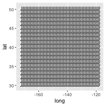
## 曲线
#### 参数:x,xend,y,yend,alpha,angle,color,curvature,linetype,size
b + geom_curve(aes(yend = lat + 1, xend=long+1,curvature=z))
## Warning: Ignoring unknown aesthetics: curvature
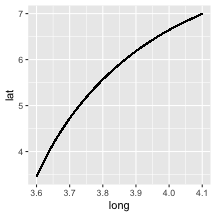
1
b + geom_curve(aes(x =4.1,y = 7,yend =3.46,xend = 3.6),curvature=0.2)
1
2
3
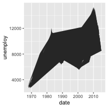
## 路径
#### 参数:x,y,alpha,color,group,linetype,size
a + geom_path(lineend="butt",linejoin = "round",linemitre = 1)

1
2
3
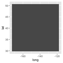
## 多边形
#### 参数:x,y,alpha,color,fill,group,linetype,size
a + geom_polygon(aes(group = psavert))
1
2
3
## 长方形
#### 参数:xmax, xmin, ymax, ymin, alpha, color, fill, linetype, size
b + geom_rect(aes(xmin = long, ymin=lat, xmax= long + 1, ymax = lat + 1))
1
2
3
## 丝带
#### 参数:x, ymax, ymin, alpha, color, fill, group, linetype, size
a + geom_ribbon(aes(ymin=unemploy - 900, ymax=unemploy + 900))
2.线条图
1
2
3
#### 参数:x, y, alpha, color, linetype, size
## 任意线
b + geom_abline(aes(intercept=0, slope=1))
1
2
## 水平线
b + geom_hline(aes(yintercept = lat))

1
2
## 垂直线
b + geom_vline(aes(xintercept = long))
1
2
## 分割线
b + geom_segment(aes(yend=lat+1, xend=long+1))
1
2
## 条幅线
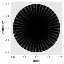
a + geom_spoke(aes(x=1,y=1,angle = 1:574, radius = 0.2))
3.单一变量
1
2
3
4
5
6
7
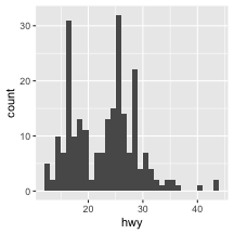
c <- ggplot(mpg,aes(hwy))
c2 <- ggplot(mpg)
##### 连续型变量
## 面积图
#### 参数:x, y, alpha, color, fill, linetype, size
c + geom_area(stat = "bin")
## `stat_bin()` using `bins = 30`. Pick better value with `binwidth`.
1
2
3
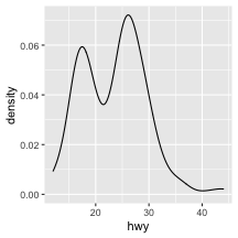
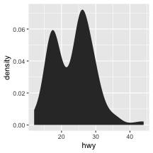
## 密度图
#### 参数:x, y, alpha, color, fill, group, linetype, size, weight
c + geom_density(kernel = "gaussian")
1
2
3
4
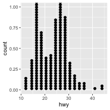
## 圆点图
#### 参数:x, y, alpha, color, fill
c + geom_dotplot()
## Bin width defaults to 1/30 of the range of the data. Pick better value with `binwidth`.
1
2
3
4
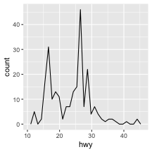
## 频率多边形图
#### 参数:x, y, alpha, color, group, linetype, size
c + geom_freqpoly()
## `stat_bin()` using `bins = 30`. Pick better value with `binwidth`.
1
2
3
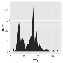
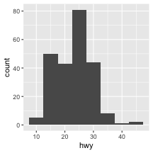
## 直方图
#### 参数:x, y, alpha, color, fill, linetype, size, weight
c + geom_histogram(binwidth = 5)
1
2
3
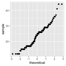
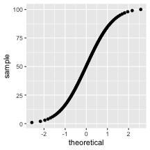
## qq图
#### 参数:x, y, alpha, color, fill, linetype, size, weight
c2 + geom_qq(aes(sample = hwy))
1
2
3
4
5
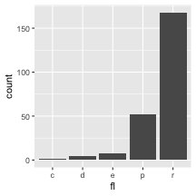
##### 非连续型变量
d <- ggplot(mpg, aes(fl))
## 柱状图
#### 参数: x, alpha, color, fill, linetype, size, weight
d + geom_bar()
4.双变量
- 连续型x,连续型y
1
2
3
4
5
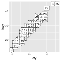
e <- ggplot(mpg,aes(cty,hwy))
## 标记图
####参数:x, y, label, alpha, angle, color, family, fontface, hjust, lineheight, size, vjust
e + geom_label(aes(label = cty), nudge_x = 1, nudge_y = 1, check_overlap = TRUE)
## Warning: Ignoring unknown parameters: check_overlap
1
2
3
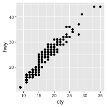
## 抖动图
####参数:x, y, alpha, color, fill, shape, size
e + geom_jitter(height = 2, width = 2)
1
2
3
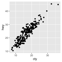
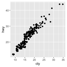
## 散点图
####参数: x, y, alpha, color, fill, shape, size, stroke
e + geom_point()
1
2
3
4
## 分位图
####参数:x, y, alpha, color, group, linetype, size, weight
e + geom_quantile()
## Smoothing formula not specified. Using: y ~ x
1
2
3
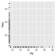
## 轴须图
####参数:x, y, alpha, color, linetype, size
e + geom_rug(sides = "bl")
1
2
3
4
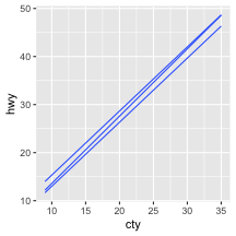
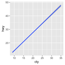
## 平滑曲线图
####参数:x, y, alpha, color, fill, group, linetype, size, weight
e + geom_smooth(method = lm)
## `geom_smooth()` using formula 'y ~ x'
1
2
3
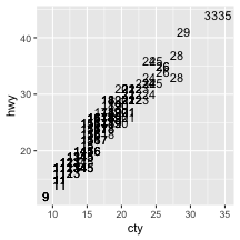
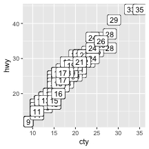
## 文字标记图
####参数:nudge_x = 1, nudge_y = 1, check_overlap = TRUE), x, y, label, alpha, angle, color, family, fontface, hjust, lineheight, size, vjust
e + geom_text(aes(label = cty))
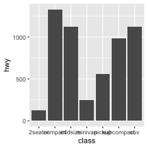
- 不连续型x,连续型y
1
2
3
4
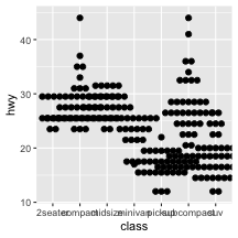
f <- ggplot(mpg, aes(class, hwy))
## 因子变量的柱状图
####参数:x, y, alpha, color, fill, group, linetype, size
f + geom_col()
1
2
3
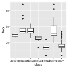
## 盒形图(箱型图)
####参数:x, y, lower, middle, upper, ymax, ymin, alpha, color, fill, group, linetype, shape, size, weight
f + geom_boxplot()

1
2
3
4
## 因子变量的圆点图
####参数:x, y, alpha, color, fill, group
f + geom_dotplot(binaxis = "y", stackdir = "center")
## Bin width defaults to 1/30 of the range of the data. Pick better value with `binwidth`.
1
2
3
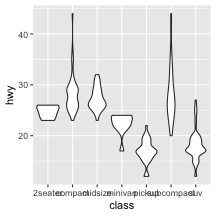
## 小提琴图
####参数:x, y, alpha, color, fill, group, linetype, size, weight
f + geom_violin(scale = "area")

- 不连续型x,不连续型y
1
2
3
4
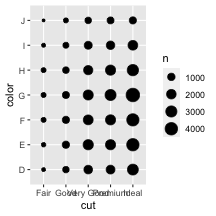
g <- ggplot(diamonds, aes(cut, color))
## 计数图
####参数:x, y, alpha, color, fill, shape, size, stroke
g + geom_count()
1
2
3
4
5
6
##### 连续型二维变量(区域密度图)
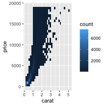
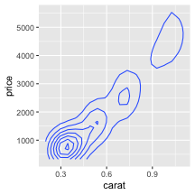
h <- ggplot(diamonds, aes(carat, price))
## 区间密度图(bin2d)
####参数:x,y,alpha,color,fill,linetype,size,weight
h + geom_bin2d(bingwidth = c(0.25,500))
## Warning: Ignoring unknown parameters: bingwidth
1
2
3
## 密度曲线图
####参数:x,y,alpha,color,group,linetype,size
h + geom_density2d()
1
2
3
## 区间密度六边形图(hex)
####参数:x,y,alpha,color,fill,size
h + geom_hex()

- 功能连续型
1
2
3
4
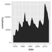
i <- ggplot(economics,aes(date,unemploy))
## 面积
####参数:x,y,alpha,color,fill,linetype,size
i + geom_area()
1
2
3
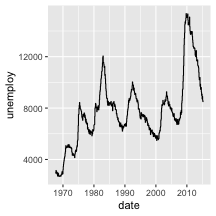
## 线状图
####参数:x,y,alpha,color,group,linetype,size
i + geom_line()

1
2
3
## 阶梯图
####参数:x,y,alpha,color,group,linetype,size
i + geom_step(direction = "hv")
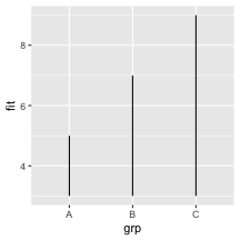
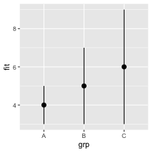
- 带误差值的图(error bar)
1
2
3
4
5
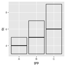
df <- data.frame(grp = c("A","B","C"),fit = 4:6,se = 1:3)
j <- ggplot(df,aes(grp,fit,ymin=fit-se,ymax=fit+se))
## 带状图
####参数:x, y, ymax, ymin, alpha, color, fill, group, linetype, size
j + geom_crossbar(fatten = 2)
1
2
3
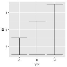
## 误差棒图 (errorbar || errorbarh)
####参数:x, y, ymax, ymin, alpha, color, fill, group, linetype, size, width
j + geom_errorbar()
1
2
3
## 线段区间图
####参数:x, y, ymax, ymin, alpha, color, fill, group, linetype, size
j + geom_linerange()
1
2
3
## 点线区间图
####参数:x, y, ymax, ymin, alpha, color, fill, group, linetype, size, shape
j + geom_pointrange()
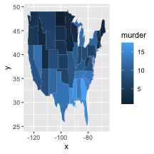
- 地图(map)
1
2
3
4
5
6
7
data <- data.frame(murder = USArrests$Murder,
                   state = tolower(rownames(USArrests)))
map <- map_data("state")
k <- ggplot(data, aes(fill = murder))
## 地图
####参数:map_id, alpha, color, fill, linetype, size
k + geom_map(aes(map_id = state), map = map) + expand_limits(x = map$long, y = map$lat)
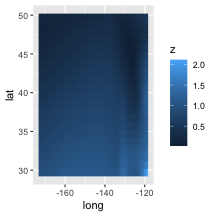
5.三变量
1
2
3
4
5
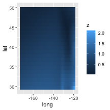
seals$z <- with(seals,sqrt(delta_long^2+delta_lat^2))
l <- ggplot(seals, aes(long, lat))
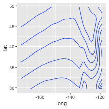
## 等高线图(contour)
####参数:x, y, z, alpha, colour, group, linetype, size, weight
l + geom_contour(aes(z = z))

1
2
3
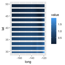
## 栅格图 (raster)
####参数:x, y, alpha, fill
l + geom_raster(aes(fill = z), hjust=0.5, vjust=0.5, interpolate=FALSE)
1
2
3
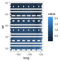
## 瓦片图 (tile)
####参数:x, y, alpha, color, fill, linetype, size, width
l + geom_tile(aes(fill = z))
统计(stats)
+ (aes( = ),geom = ) i + stat_density2d(aes(fill = level),geom = "polygon")
1
2
3
4
5
6
7
##数据准备
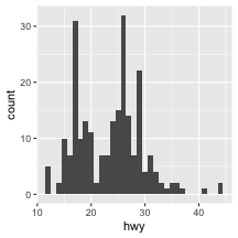
c <- ggplot(mpg, aes(hwy))
e <- ggplot(mpg, aes(cty, hwy))
seals$z <- with(seals, sqrt(delta_long^2 + delta_lat^2))
l <- ggplot(seals, aes(long, lat))
f <- ggplot(mpg, aes(class, hwy))
h <- ggplot(diamonds, aes(carat, price))
- 统计落在x(连续)区间上,点的个数
1
2
#### x, y | ..count.., ..ncount.., ..density.., ..ndensity..
c + stat_bin(binwidth = 1, origin = 10)
- 统计落在x(离散)位置上,点的个数
1
2
#### x, y, | ..count.., ..prop..
c + stat_count(width = 1)
- x(连续)核密度估计,可以看作是直方图的平滑版本
1
2
#### x, y, | ..count.., ..density.., ..scaled..
c + stat_density(adjust = 1, kernel = "gaussian")
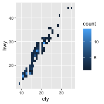
- 统计落在x和y(长方形)区域上点的个数
1
2
####x, y, fill | ..count.., ..density..
e + stat_bin_2d(bins = 30, drop = T)
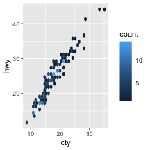
- 统计落在六边形区域上点的个数,stat_bin2d()的六边形版本
1
2
#### x, y, fill | ..count.., ..density..
e + stat_bin_hex(bins=30)
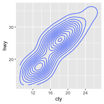
- 二维核密度估计,二维版本的stat_density()
1
2
#### x, y, color, size | ..level..
e + stat_density_2d(contour = TRUE, n = 100)
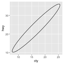
- 假定数据服从多元分布,计算椭圆图形需要的参数
1
e + stat_ellipse(level = 0.95, segments = 51, type = "t")
- 等高线、等高面,需要提供x,y,z映射
1
2
#### x, y, z, order | ..level..
l + stat_contour(aes(z = z))
- 落在x和y(六边形)区域上, summary on z
1
2
#### x, y, z, fill | ..value..
l + stat_summary_hex(aes(z = z), bins = 30, fun = max)
- 落在x和y(长方形)区域上, summary on z
1
2
#### x, y, z, fill | ..value..
l + stat_summary_2d(aes(z = z), bins = 30, fun = mean)
- 计算连续变量的五个统计值 (the median, two hinges and two whiskers), 以及outlier
1
2
#### x, y | ..lower.., ..middle.., ..upper.., ..width.. , ..ymin.., ..ymax..
f + stat_boxplot(coef = 1.5)
- 箱线图的密度图呈现
1
2
#### x, y | ..density.., ..scaled.., ..count.., ..n.., ..violinwidth.., ..width..
f + stat_ydensity(kernel = "gaussian", scale = "area")
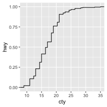
- 统计经验累积分布
1
2
#### x, y | ..x.., ..y..
e + stat_ecdf(n = 40)
- 分位数回归
1
2
#### x, y | ..quantile..
e + stat_quantile(quantiles = c(0.1, 0.9), formula = y ~ log(x), method = "rq")
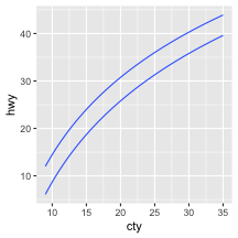
- 根据x,y数据和拟合公式,计算每个点位置的拟合值以及标准误
1
2
#### x, y | ..se.., ..x.., ..y.., ..ymin.., ..ymax..
e + stat_smooth(method = "lm", formula = y ~ x, se=T, level=0.95)

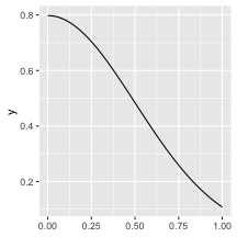
- 叠加自定义函数
1
2
3
#### x | ..x.., ..y..
x = runif(n = 100, min = -5, max = 5)
ggplot() + stat_function(n = 99, fun = dnorm, args = list(mean = 0, sd = 0.5))
- 等值转换
1
e + stat_identity(na.rm = TRUE)

- qq 分位数图的统计
1
2
#### sample, x, y | ..sample.., ..theoretical..
ggplot() + stat_qq(aes(sample=1:100), dist = qt, dparam=list(df=5))
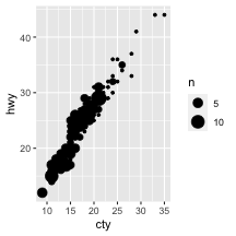
- 统计落在x(连续), y(连续)位置上,点的个数
1
2
#### x, y, size | ..n.., ..prop..
e + stat_sum()
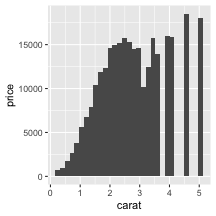
- 每一个x位置上, summary on y
1
e + stat_summary(fun.data = "mean_cl_boot")
- 在落入x区间位置上的y,设定函数(也可以调整方向,对落入y区间位置的每个x,设定函数)
1
h + stat_summary_bin(fun.y = "mean", geom = "bar")
- 移除重复值
1
e + stat_unique()

范围(scales)
- 组成结构
scale_aesthetic to adjust_prepackaged scale to use( values,limits,breaks,name,labels )
1
2
3
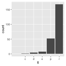
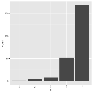
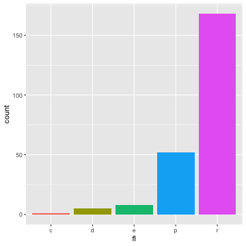
d <- ggplot(mpg, aes(fl))
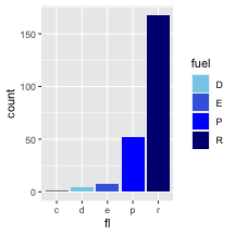
n <- d + geom_bar(aes(fill = fl))
n + scale_fill_manual( values = c("skyblue", "royalblue", "blue", "navy"), limits = c("d", "e", "p", "r"), breaks =c("d", "e", "p","r"), name = "fuel", labels = c("D", "E", "P", "R"))
- 基本类型
| 形式 | 描述 |
|---|---|
| scale_&_continous() | 连续型变量 |
| scale_&_discrete() | 离散型变量 |
| scale_&_identity() | 单独变量 |
| scale_&_manual() | 使用指定值 |
| scale_&_date() | 数据转换为时间 |
| scale_&_datetime() | 数据转换为时间 |
- x,y 的位置变换
| 形式 | 描述 |
|---|---|
| scale_x_log10() | 取log10 |
| scale_x_reverse() | 取倒数 |
| scale_x_sqrt() | 取开方 |
- 颜色转换
1
2
3
4
#### 离散
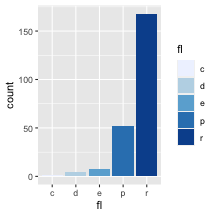
n <- d + geom_bar(aes(fill = fl))
## 色彩渐变
n + scale_fill_brewer(palette = "Blues")
1
2
3
#### For palette choices: RColorBrewer::display.brewer.all()
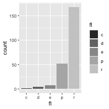
## 灰度
n + scale_fill_grey(start = 0.2, end = 0.8, na.value = "red")
1
2
3
4
5
6
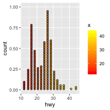
#### 连续
##
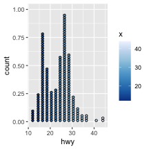
o <- c + geom_dotplot(aes(fill = ..x..))
o + scale_fill_distiller(palette = "Blues")
## Bin width defaults to 1/30 of the range of the data. Pick better value with `binwidth`.
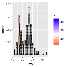
1
2
o + scale_fill_gradient(low="red", high="yellow")
## Bin width defaults to 1/30 of the range of the data. Pick better value with `binwidth`.
1
2
o + scale_fill_gradient2(low="red", high="blue", mid = "white", midpoint = 25)
## Bin width defaults to 1/30 of the range of the data. Pick better value with `binwidth`.
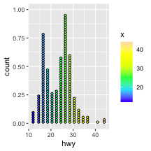
1
2
o + scale_fill_gradientn(colours=topo.colors(6))
## Bin width defaults to 1/30 of the range of the data. Pick better value with `binwidth`.
1
#### Also: rainbow(), heat.colors(), terrain.colors(), cm.colors(), RColorBrewer::brewer.pal()
- 图形与大小
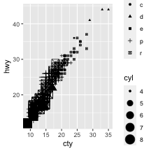
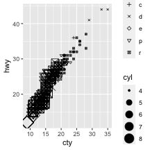
1
2
p <- e + geom_point(aes(shape = fl, size = cyl))
p + scale_shape() + scale_size()
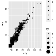
1
p + scale_shape_manual(values = c(3:7))
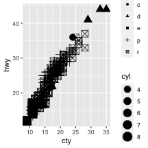
1
p + scale_radius(range = c(1,6))
1
p + scale_size_area(max_size = 6)
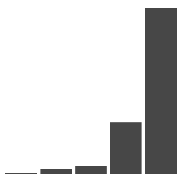
坐标轴系统(coordinate)
1
2
3
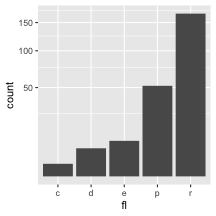
r <- d + geom_bar()
## 默认笛卡尔坐标系统
r + coord_cartesian(xlim = c(0, 5))
1
2
## y,x 比例扩缩
r + coord_fixed(ratio = 1/2)
1
2
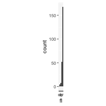
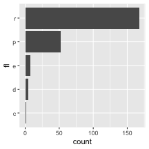
## y,x 交换
r + coord_flip()
1
2
3
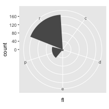
## 极坐标
#### theta, start, direction Polar coordinates
r + coord_polar(theta = "x", direction=1)
1
2
3
## 函数式转换
#### x, y, limx, limy
r + coord_trans(y = "sqrt")
1
2
3
4
5
6
## 地图系统
#### projection, orienztation, xlim, ylim Map projections from the mapproj package (mercator (default), azequalarea, lagrange, etc.)
π + coord_quickmap()
## Error in eval(expr, envir, enclos): object '\u03c0' not found
π + coord_map(projection = "ortho", orientation=c(41, -74, 0))
## Error in eval(expr, envir, enclos): object '\u03c0' not found
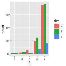
位置(position)
1
2
3
s <- ggplot(mpg, aes(fl, fill = drv))
## 紧靠
s + geom_bar(position = "dodge")
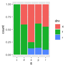
1
2
## 百分比堆叠
s + geom_bar(position = "fill")
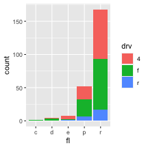
1
2
## 绝对值堆叠
s + geom_bar(position = "stack")
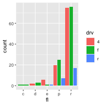
1
2
## 相隔位置
s + geom_bar(position = position_dodge(width = 1))
1
2
## 随机抖动
e + geom_point(position = "jitter")
1
2
##
e + geom_label(aes(label = cty),position = "Nudge")
分组(facets)
1
2
3
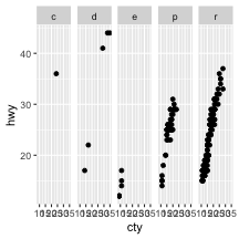
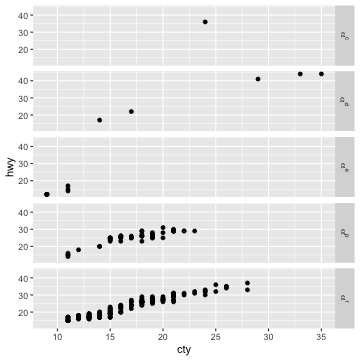
t <- ggplot(mpg, aes(cty, hwy)) + geom_point()
## 以列分组
t + facet_grid(cols = vars(fl))
1
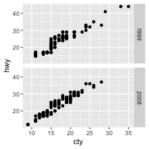
2
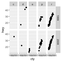
## 以行分组
t + facet_grid(rows = vars(year))
1
2
## 以格子分组
t + facet_grid(rows = vars(year), cols = vars(fl))
1
2
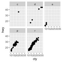
## 以某个变量分组
t + facet_wrap(vars(fl))
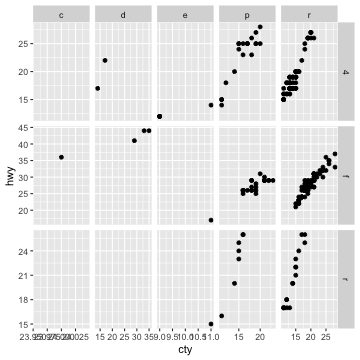
设置“free”变量来更改x,y轴的范围
1
t + facet_grid(rows = vars(drv), cols = vars(fl), scales = "free")
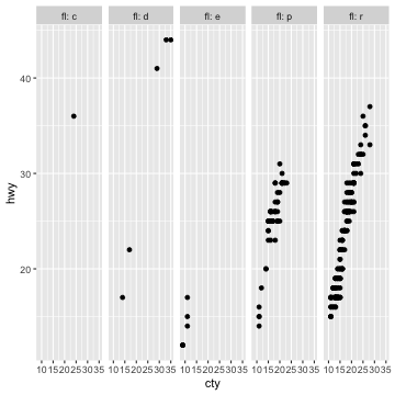
设置“labeller”变量来更改x,y轴的标签
1
t + facet_grid(cols = vars(fl), labeller = label_both)
1
t + facet_grid(rows = vars(fl), labeller = label_bquote(alpha ^ .(fl)))
主题(Theme)
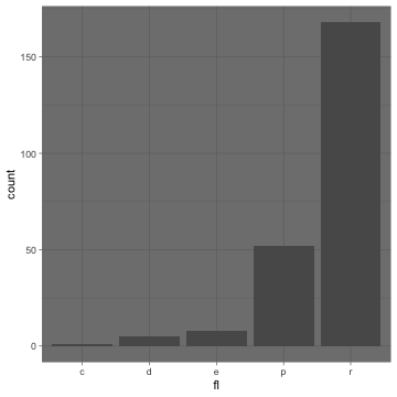
1
r + theme_bw()

1
r + theme_gray()
1
r + theme_dark()
1
r + theme_classic()

1
r + theme_light()

1
r + theme_linedraw()
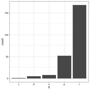
1
r + theme_minimal()

1
r + theme_void()
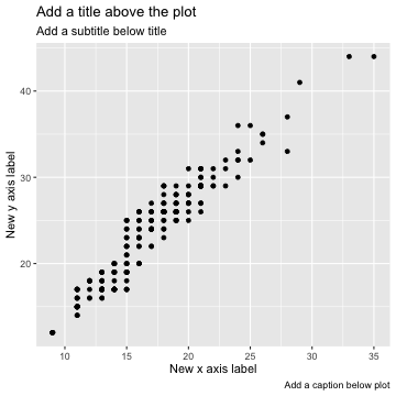
标记(label)
1
2
3
4
5
t + labs( x = "New x axis label", y = "New y axis label",
          title ="Add a title above the plot",
          subtitle = "Add a subtitle below title",
          caption = "Add a caption below plot",
          labels = "New legend title")
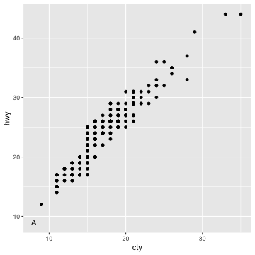
1
2

t + annotate(geom = "text", x = 8, y = 9, label = "A")
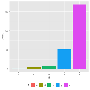
图例
1
2
### Place legend at "bottom", "top", "left", or "right"
n + theme(legend.position = "bottom")
1
2
### Set legend type for each aesthetic: colorbar, legend, or none (no legend)
n + guides(fill = "none")
1
2
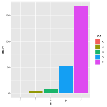
### 使用scale做图例的标题和标记
n + scale_fill_discrete(name = "Title", labels = c("A", "B", "C", "D", "E"))
放大(Zoom)
1
2
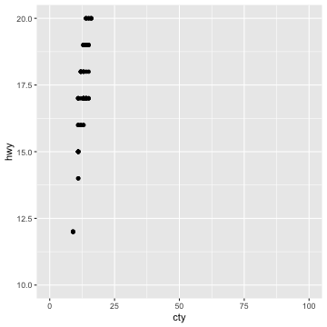
### 不剪切
t + coord_cartesian(xlim = c(0, 100), ylim = c(10, 20))

1
2
### 剪切
t + xlim(0, 100) + ylim(10, 20)
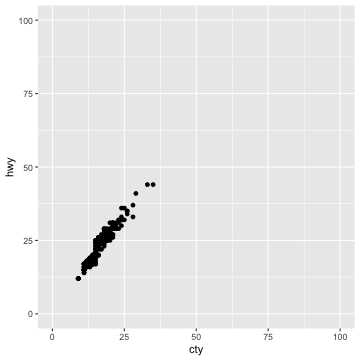
1
t + scale_x_continuous(limits = c(0, 100)) + scale_y_continuous(limits = c(0, 100))
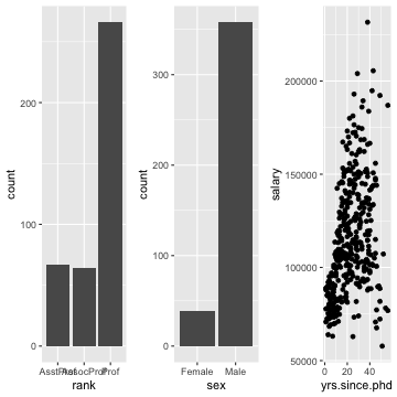
组合
1
2
3
4
5
6
7
data("Salaries",package = "car")
p1 <- ggplot(data = Salaries,aes(x = rank)) + geom_bar()
p2 <- ggplot(data = Salaries,aes(x = sex)) + geom_bar()
p3 <- ggplot(data = Salaries,aes(x = yrs.since.phd,y=salary)) + geom_point()

library(gridExtra)
grid.arrange(p1,p2,p3,ncol=3)
持续更新 。。。