段首语
此系列文章用来做R语言的学习,以及对于使用R语言进行数据处理和作图的代码汇总,方便大家随时进行查找、使用。
一、help
获取注解
- 获取某个功能(function)的具体使用
1
?mean
- 获取某个短语,文件,或者词组的具体解释
1
help.search('weighted mean')
- 获取某个R包的具体使用
1
help(package = 'dplyr')
- 获取某个变量的属性
1
2
str(iris)
class(iris)
二、包的使用
1
2
3
4
5
6
7
8
## 包的安装
install.packages("ggplot2")
## 包的使用
library(ggplot2)
## 包内具体功能的使用
dplyr::select
## 导入数据
data(iris)
三、工作目录
1
2
3
4
## 获取目录
getwd()
## 更改目录
setwd(dir = "./")
四、数据结构
1.向量(Vector)
创建
| 函数 | 变量 | 描述 |
|---|---|---|
| c(2,4,6) | 2 4 6 | 新建向量 |
| 2:6 | 2 3 4 5 6 | 有序连续整数向量 |
| seq(2,3,by=0.5) | 2.0 2.5 3.0 | 指定间隔向量 |
| rep(1:2,times=3 | 1 2 1 2 1 2 | 向量重复 |
| rep(1:2,each=3) | 1 1 1 2 2 2 | 向量元素重复 |
选择
1
2
3
4
5
6
7
8
9
10
11
12
13
14
15
16
17
18
19
20
21
22
23
24
25
x <- 1:10
# 按位置选择元素
x[4]
## [1] 4
x[2:4]
## [1] 2 3 4
# 按位置去除元素
x[-4]
## [1]  1  2  3  5  6  7  8  9 10
x[-(2:4)] ## 不包含第二到第四
## [1]  1  5  6  7  8  9 10
x[c(1,5)] ## 不包含第一和第五
## [1] 1 5
# 选择特定值的元素
x[x==10]
## [1] 10
x[x<0]
## integer(0)
subset(x,x>5)
## [1]  6  7  8  9 10
x[x %in% c(1,2,5)]
## [1] 1 2 5
# 选择特定名称的元素
x['apple']
## [1] NA
基本功能
1
2
3
4
5
6
7
8
9
10
11
12
13
14
15
16
17
18
19
20
21
22
23
24
x <- c(1,3,2,4,5,5,6,8,9,10)
x1 <- rep(1:2,times = 5)
sort(x) ## 排序
##  [1]  1  2  3  4  5  5  6  8  9 10
rev(x) ## 翻转
##  [1] 10  9  8  6  5  5  4  2  3  1
table(x) ## 查看每个元素的数目
## x
##  1  2  3  4  5  6  8  9 10
##  1  1  1  1  2  1  1  1  1
unique(x) ## 去重复
## [1]  1  3  2  4  5  6  8  9 10
x + x1 ## 加
##  [1]  2  5  3  6  6  7  7 10 10 12
x - x1 ## 减
##  [1] 0 1 1 2 4 3 5 6 8 8
x * x1 ## 乘
##  [1]  1  6  2  8  5 10  6 16  9 20
x / x1 ## 除
##  [1] 1.0 1.5 2.0 2.0 5.0 2.5 6.0 4.0 9.0 5.0
all(x > 0) ## 判断是否都满足
## [1] TRUE
any(x < 8) ## 判断是否有一个满足
## [1] TRUE
基本函数
1
2
3
4
5
6
7
8
9
10
11
12
13
14
15
16
17
18
19
20
21
22
23
24
25
26
27
28
29
30
31
32
33
34
35
36
37
sum(x) ## 求和
## [1] 53
mean(x) ## 平均值
## [1] 5.3
median(x) ## 中值
## [1] 5
quantile(x) ## 分位数
##    0%   25%   50%   75%  100%
##  1.00  3.25  5.00  7.50 10.00
rank(x) ## 排序index
##  [1]  1.0  3.0  2.0  4.0  5.5  5.5  7.0  8.0  9.0 10.0
var(x) ## 方差
## [1] 8.9
sd(x) ## 标准差
## [1] 2.983287
cumsum(x) ## 按项递加求和
##  [1]  1  4  6 10 15 20 26 34 43 53
log(x) ## log 以e为底
##  [1] 0.0000000 1.0986123 0.6931472 1.3862944 1.6094379
##  [6] 1.6094379 1.7917595 2.0794415 2.1972246 2.3025851
exp(x) ## 指数 以e为底
##  [1]     2.718282    20.085537     7.389056
##  [4]    54.598150   148.413159   148.413159
##  [7]   403.428793  2980.957987  8103.083928
## [10] 22026.465795
max(x)
## [1] 10
min(x)
## [1] 1
q <- c(1.2214,1.3324,1.4423)
round(q,3) ## 保留位数
## [1] 1.221 1.332 1.442
signif(q,2) ## 精确度
## [1] 1.2 1.3 1.4
y <- rev(x)
cor(x,y) ## 相关性
## [1] -0.9600499
2.矩阵和数组
创建
- 矩阵
1
2
3
4
5
6
7
8
9
10
c <- seq(1,9)
namerow <- c("R1","R2","R3")
namecol <- c("C1","C2","C3")
m <- matrix(c,nrow=3,ncol=3,byrow = TRUE,dimnames = list(namerow,namecol))
m
##    C1 C2 C3
## R1  1  2  3
## R2  4  5  6
## R3  7  8  9
## nrow 行数 ncol 列数 byrow 按行填充还是按列填充,dimnames(行列名)
- 数组
1
2
3
4
5
6
7
8
9
10
11
12
13
14
15
16
17
18
19
20
21
22
23
24
25
26
27
28
29
## myarray <- array(vector,dimension,dimnames)
dim1 <- c("A1","A2")
dim2 <- c("B1","B2","B3")
dim3 <- c("C1","C2","C3","C4")
z <- array(1:24,c(2,3,4),dimnames = list(dim1,dim2,dim3))
z
## , , C1
##
##    B1 B2 B3
## A1  1  3  5
## A2  2  4  6
##
## , , C2
##
##    B1 B2 B3
## A1  7  9 11
## A2  8 10 12
##
## , , C3
##
##    B1 B2 B3
## A1 13 15 17
## A2 14 16 18
##
## , , C4
##
##    B1 B2 B3
## A1 19 21 23
## A2 20 22 24
对矩阵的行和列调用函数
apply(m,dimcode,f,fargs)
- m代表矩阵
- dimcode代表维度编号,1代表对每一行应用函数,2代表对每一列应用函数
- f使用的函数运算(循环补齐)
- fargs f函数可调用的参数
1
2
3
4
5
6
7
8
9
10
11
12
13
14
15
16
17
18
19
z <- matrix(1:6,nrow=3,ncol=2)
z
##      [,1] [,2]
## [1,]    1    4
## [2,]    2    5
## [3,]    3    6
apply(z,1,mean)
## [1] 2.5 3.5 4.5
f<- function(x) {x/c(2,8)}
apply(z,2,f)
## Warning in x/c(2, 8): longer object length is not a
## multiple of shorter object length

## Warning in x/c(2, 8): longer object length is not a
## multiple of shorter object length
##      [,1]  [,2]
## [1,] 0.50 2.000
## [2,] 0.25 0.625
## [3,] 1.50 3.000
矩阵的组合
1
2
3
4
5
6
7
8
9
10
11
cbind(1,z) ## 行不变,列增加
##      [,1] [,2] [,3]
## [1,]    1    1    4
## [2,]    1    2    5
## [3,]    1    3    6
rbind(1,z) ## 列不变,行增加
##      [,1] [,2]
## [1,]    1    1
## [2,]    1    4
## [3,]    2    5
## [4,]    3    6
3.列表
创建
1
2
3
4
5
6
7
8
9
10
j <- list(name="Joe",salary = 55000,union=T)
j
## $name
## [1] "Joe"
##
## $salary
## [1] 55000
##
## $union
## [1] TRUE
常用操作
1
2
3
4
5
6
7
8
## 索引
j$salary
j[1]
## 增删
j$age <- 45
j$union <- NULL
## 访问元素
unlist(j)
4.数据框
创建
mydata <- data.frame(col1,col2,col3)
1
2
3
4
5
6
7
8
9
10
11
patientID <- c(1,2,3,4)
age <- c(25,34,28,51)
diabetes <- c("Type1","Type2","Type1","Type1")
status <- c("Poor","Improved","Excellent","Poor")
patientData <- data.frame(patientID,age,diabetes,status)
patientData
##   patientID age diabetes    status
## 1         1  25    Type1      Poor
## 2         2  34    Type2  Improved
## 3         3  28    Type1 Excellent
## 4         4  51    Type1      Poor
基本操作
- attach() 添加到R的搜索路径中
- detach() 从搜索路径中解除
- with()
1
2
3
4
5
6
7
8
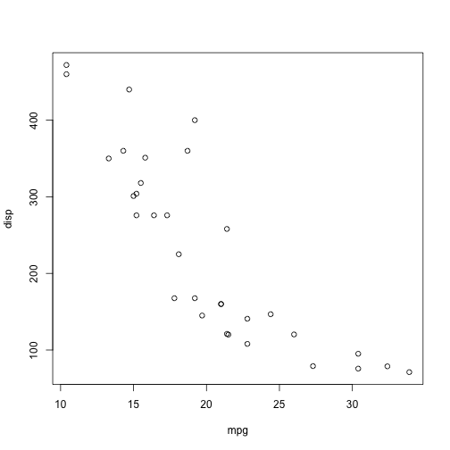
attach(mtcars)
## The following object is masked from package:ggplot2:
##
## mpg
summary(mpg)
## Min. 1st Qu. Median Mean 3rd Qu. Max.
## 10.40 15.43 19.20 20.09 22.80 33.90
plot(mpg,disp)
1
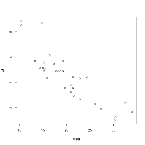
plot(mpg,wt)
1
detach(mtcars)
类似于矩阵的操作
- cbind()
- rbind()
- dim()
- subset()
- apply()
数据框的合并
merge()
merge(x, y, by = intersect(names(x), names(y)), by.x = by, by.y = by, all = FALSE, all.x = all, all.y = all, sort = TRUE, suffixes = c(“.x”,”.y”), no.dups = TRUE, incomparables = NULL, …)
1
2
3
4
5
6
7
8
9
10
11
12
13
14
15
16
17
18
19
20
21
22
23
24
25
26
27
28
29
30
31
d1 <- data.frame(kids=c("Jack","Jill","Jillian","John"),states = c("CA","MA","MA","HI"))
d1
##      kids states
## 1    Jack     CA
## 2    Jill     MA
## 3 Jillian     MA
## 4    John     HI
d2 <- data.frame(ages=c(10,7,12),kids=c("Jill","Lillian","Jack"))
d2
##   ages    kids
## 1   10    Jill
## 2    7 Lillian
## 3   12    Jack
merge(d1,d2)
##   kids states ages
## 1 Jack     CA   12
## 2 Jill     MA   10
merge(d1,d2,by.x="kids")
##   kids states ages
## 1 Jack     CA   12
## 2 Jill     MA   10
merge(d1,d2,by.y = "ages")
## [1] kids   states kids.y
## <0 rows> (or 0-length row.names)
merge(d1,d2,all=T)
##      kids states ages
## 1    Jack     CA   12
## 2    Jill     MA   10
## 3 Jillian     MA   NA
## 4    John     HI   NA
## 5 Lillian   <NA>    7
5.因子
1
2
3
4
5
6
7
8
status
## [1] "Poor"      "Improved"  "Excellent" "Poor"
factor(status)
## [1] Poor      Improved  Excellent Poor
## Levels: Excellent Improved Poor
factor(status,ordered=TRUE,levels = c("Poor","Improved","Excellent"))
## [1] Poor      Improved  Excellent Poor
## Levels: Poor < Improved < Excellent
tapply
和apply类似,分组使用了因子的不同水平为标准
1
2
3
4
5
ages <- c(25,26,55,37,21,42)
affils <- c("R","D","D","R","U","D")
tapply(ages,affils,mean)
##  D  R  U
## 41 31 21
6.String
x <- c(“I”,”M”)
y <- c(“P”,”C”)
| Strings | results |
|---|---|
| paste(x,y,sep =’ ‘) | “I P” “M C” |
| paste(x,collapse=’ ‘) | “I M” |
| grep(“M”,x) | 2 |
| gsub(“M”,”A”,x) | “I” “A” |
| toupper(x) | “I” “M” |
| tolower(x) | “i” “m” |
| nchar(x) | 1 1 |
五、其他数据操作
1.缺失值的管理
1
2
3
4
5
6
7
8
9
10
11
y <- c(1,2,3,NA)
is.na(y) ## 判断缺失值
## [1] FALSE FALSE FALSE  TRUE
sum(y,na.rm = T) ## 排除缺失值
## [1] 6
leadership <- data.frame(manager=c(1,2,3,4,5),gender = c("M","F","F","M","F"),q1=c(5,2,3,NA,1),q2=c(1,2,NA,3,4))
na.omit(leadership) ## 删除不完整的观测,数据框中删除带有NA的行
##   manager gender q1 q2
## 1       1      M  5  1
## 2       2      F  2  2
## 5       5      F  1  4
2.概率函数
| 分布名称 | 缩写 |
| Beta分布 | beta |
| 二项分布 | binom |
| 柯西分布 | cauchy |
| (非中心)卡方分布 | chisq |
| 指数分布 | exp |
| F分布 | f |
| Gamma分布 | gamma |
| 几何分布 | geom |
| 超几何分布 | hyper |
| 对数正态分布 | lnorm |
| Logistic分布 | logis |
| 多项分布 | multinom |
| 负二项分布 | nbinom |
| 正态分布 | norm |
| 泊松分布 | pois |
| Wilcoxon符号秩分布 | signrank |
| t分布 | t |
| 均匀分布 | unif |
| Weibull分布 | weibull |
| Wilcoxon秩和分布 | wilcox |
1
2
3
4
5
6
7
8
9
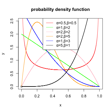
x<-seq(0,1,length.out=10000)
plot(0,0,main='probability density function',xlim=c(0,1),ylim=c(0,2.5),ylab='y',xlab = 'x')
lines(x,dbeta(x,0.5,0.5),col='red')
lines(x,dbeta(x,1,2),col='green')
lines(x,dbeta(x,2,2),col='pink')
lines(x,dbeta(x,2,5),col='orange')
lines(x,dbeta(x,1,3),col='blue')
lines(x,dbeta(x,5,1),col='black')
legend('top',legend=c('α=0.5,β=0.5','α=1,β=2','α=2,β=2','α=2,β=5','α=1,β=3','α=5,β=1'),col=c('red','green','pink','orange','blue','black'),lwd=1)
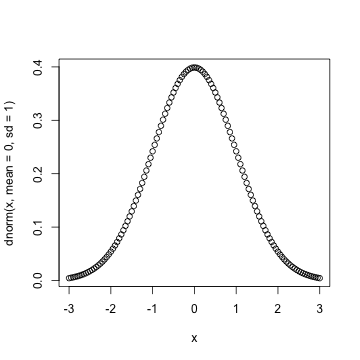
- dnorm() 密度分布
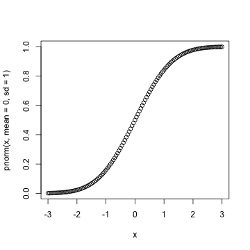
- pnorm() 分布函数
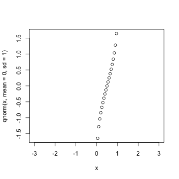
- qnorm() 分位数函数
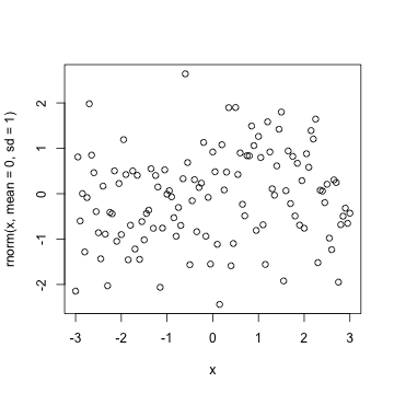
- rnorm() 生成随机数
1
2
x <- pretty(c(-3,3),100) ## 生成符合标准正态分布的随机数
plot(x,dnorm(x,mean = 0,sd = 1))
1
plot(x,pnorm(x,mean = 0,sd = 1))
1
plot(x,qnorm(x,mean = 0,sd = 1))
1
plot(x,rnorm(x,mean = 0,sd = 1))
3.控制流
- for循环 for (var in seq) statment
- while while (cond) statement
- if-else if(cond) statement1 else statement2
- 自编函数 myfunction <- function(arg1,arg2, … ){ statements return(object) }
4.reshape2包
融合
1
2
3
4
5
6
7
8
9
10
11
12
13
14
15
16
17
18
19
library(reshape2)
mydata <- data.frame(ID = c(1,1,2,2),Time=c(1,2,1,2),X1=c(5,3,6,2),X2=c(6,5,1,4))
mydata
##   ID Time X1 X2
## 1  1    1  5  6
## 2  1    2  3  5
## 3  2    1  6  1
## 4  2    2  2  4
md <- melt(mydata,id=c("ID","Time"))
md
##   ID Time variable value
## 1  1    1       X1     5
## 2  1    2       X1     3
## 3  2    1       X1     6
## 4  2    2       X1     2
## 5  1    1       X2     6
## 6  1    2       X2     5
## 7  2    1       X2     1
## 8  2    2       X2     4
重铸
1
2
3
4
5
6
7
8
9
10
11
12
13
14
15
16
17
18
19
20
21
22
23
24
25
26
27
28
29
30
31
32
33
34
35
library(reshape2)
names(airquality) <- tolower(names(airquality))
head(airquality)
##   ozone solar.r wind temp month day
## 1    41     190  7.4   67     5   1
## 2    36     118  8.0   72     5   2
## 3    12     149 12.6   74     5   3
## 4    18     313 11.5   62     5   4
## 5    NA      NA 14.3   56     5   5
## 6    28      NA 14.9   66     5   6
aqm <- melt(airquality, id=c("month", "day"), na.rm=TRUE)
head(aqm)
##   month day variable value
## 1     5   1    ozone    41
## 2     5   2    ozone    36
## 3     5   3    ozone    12
## 4     5   4    ozone    18
## 6     5   6    ozone    28
## 7     5   7    ozone    23
acast(aqm, month ~ variable, mean, margins = TRUE)
##          ozone  solar.r      wind     temp    (all)
## 5     23.61538 181.2963 11.622581 65.54839 68.70696
## 6     29.44444 190.1667 10.266667 79.10000 87.38384
## 7     59.11538 216.4839  8.941935 83.90323 93.49748
## 8     59.96154 171.8571  8.793548 83.96774 79.71207
## 9     31.44828 167.4333 10.180000 76.90000 71.82689
## (all) 42.12931 185.9315  9.957516 77.88235 80.05722
dcast(aqm, month ~ variable, mean, margins = c("month", "variable"))
##   month    ozone  solar.r      wind     temp    (all)
## 1     5 23.61538 181.2963 11.622581 65.54839 68.70696
## 2     6 29.44444 190.1667 10.266667 79.10000 87.38384
## 3     7 59.11538 216.4839  8.941935 83.90323 93.49748
## 4     8 59.96154 171.8571  8.793548 83.96774 79.71207
## 5     9 31.44828 167.4333 10.180000 76.90000 71.82689
## 6 (all) 42.12931 185.9315  9.957516 77.88235 80.05722
持续更新 。。。